This post was originally published on Linkedin on 24 April 2023.
The way constraint equation data that is used in the NEM Dispatch Engine (NEMDE) is organised and publicly disseminated is not very intuitive. This article is an attempt to demystify and make sense of how NEMDE constraint equation formulations are structured and published.
So what are constraint equations again?
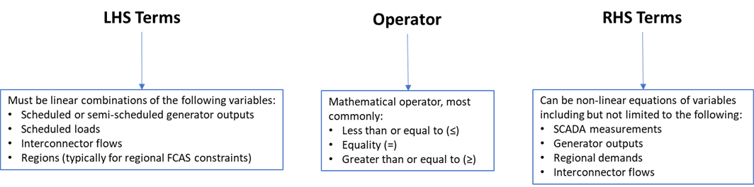
NEMDE uses linear constraints (referred to as generic constraints) to reflect physical limits in the power system that are not inherently captured in the market dispatch model, and thus prevent the system from operating outside its technical envelope. Constraints are used to represent things like network and interconnector capacity limits, stability limits, frequency control requirements, etc.
Constraints are formulated as constraint equations of the form:
For example, a very simple LHS ≤ RHS constraint formulation is the constraint equation “Q_OKYTX4”, which limits the output of Oakey 1 and 2 Solar Farms to 71 MW when there is an outage on the Oakey 4T 110/33kV transformer:
1.0 x OAKEY1SF + 1.0 x OAKEY2SF ≤ 71
Constraint equation formulations are not designed for human readability
Like most of the data in AEMO’s Market Management System (MMS), constraint equation formulations are structured for use in a relational database, such that a computer can efficiently access and query the data. So while the data is made available to the general public, it is practically inaccessible to most people as there is a significant amount of data wrangling that needs to be done. Third-party software packages (like Global-Roam’s ez2view) make this more accessible by doing all the data wrangling work behind the scenes.
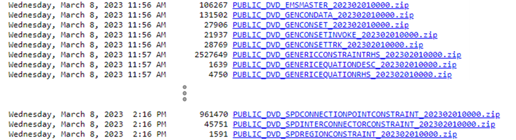
In any case, the constraint equation formulations can be found in the MMS Data Model Archive as part of the GENERIC_CONSTRAINT package. It is important to note that this archive is organised as monthly data dumps and monthly archive only shows constraint equations that were updated in that month. To access existing constraint equation formulations that haven’t changed, you have to navigate back to the month/year that it was either last modified or first created.
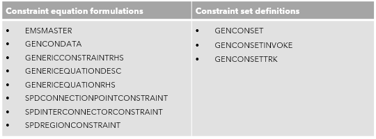
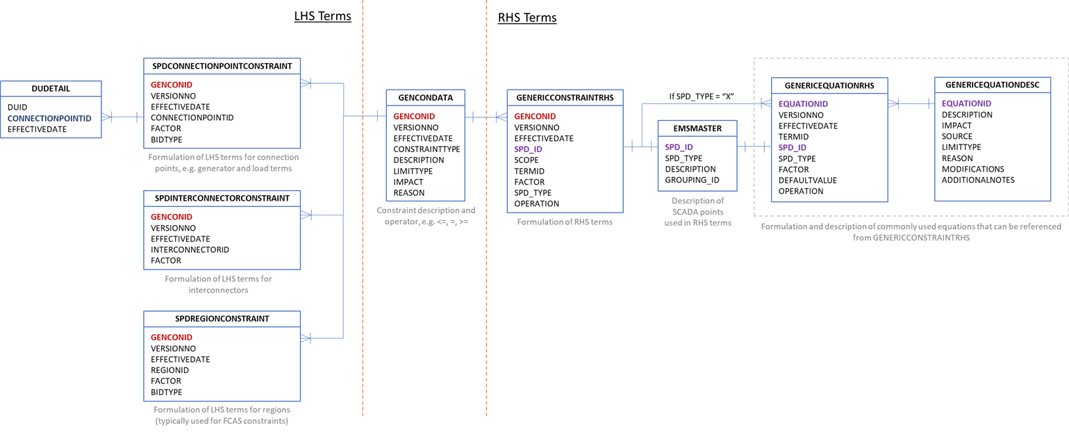
There are 8 tables that define the constraint equation formulations and 3 other tables defining constraint sets:
For example, in the February 2023 archive, these tables are shown as follows:
The relationships between the 8 constraint equation formulation tables are shown in the diagram below (which is essentially an expanded and annotated version of the diagram in section 14.2 of the MMS Data Model v5.1 Package Summary document):
A simple worked example illustrates how the tables in MMS fit together
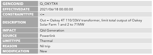
In this worked example, we will find the formulation for constraint equation “Q_OKYTX4”. This equation was last updated in June 2021, and the relevant data files can be accessed from the June 2021 MMS Data Model Archive folder.
The GENCONDATA table provides summary information about the constraint equation, including the operator for the constraint (≤).
The SPDCONNECTIONPOINTCONSTRAINT table provides the relevant LHS terms:
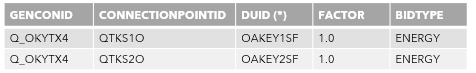
There are no other LHS terms in SPDINTERCONNECTORCONSTRAINT and SPDREGIONCONSTRAINT corresponding to constraint equation Q_OKYTX4, so the LHS is simply a linear combination of two terms:
LHS = 1.0 x OAKEY1SF + 1.0 x OAKEY2SF
The GENERICCONSTRAINTRHS table provides the relevant RHS terms, which in this case is just a constant value:
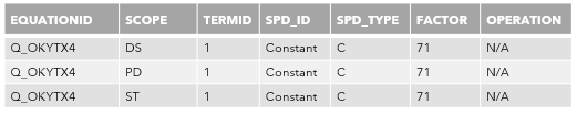
Note that the scope field determines which NEMDE run the RHS term is applicable to, i.e. DS = Dispatch, PD = Pre-dispatch (PD PASA), ST = ST PASA.
There are no cross-references to EMSMASTER, GENERICEQUATIONRHS or GENERICEQUATIONDESC tables as the RHS is just a simple constant:
RHS = 71
Putting it all together, the constraint equation formulation is as follows:
LHS ≤ RHS
1.0 x OAKEY1SF + 1.0 x OAKEY2SF ≤ 71
Python functions to make viewing constraint equation formulations easier
I wrote a Python library with the following functions to aid in wrangling constraint equation formulations (you can get the code here on GitHub):
- get_constraint_list: get a list of constraints from the archive for a specific month/year
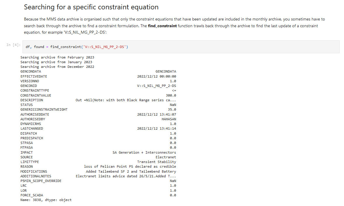
- find_constraint: search for a specific constraint equation
- get_LHS_terms: get the left-hand side (LHS) terms of a specific constraint equation
- get_RHS_terms: get the right-hand side (RHS) terms of a specific constraint equation
- get_constraint_details: get the description, LHS and RHS terms of a specific constraint equation
- find_generic_RHS_func: find a generic RHS function definition from the archive
- get_generic_RHS_func: get the terms for a generic RHS function
This Jupyter notebook provides illustrative examples of how the functions can be used. A screenshot from the notebook is shown below: